Steady or not Steady that is the question?
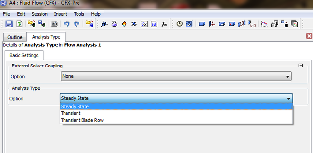
Not all numerical models in CFX produce results at a steady state, as an example you cannot run an LES simulation for a steady case the same applies to other models.
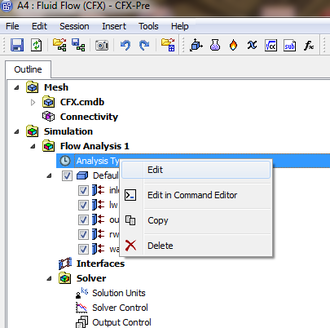
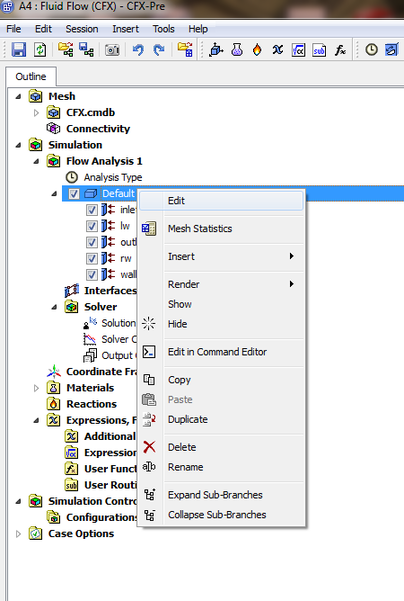
Selecting what
Unsteady Simulations
Once the researcher verify that he can run and unsteady simulation that gives correct results then comes the option of running unsteady simulations.
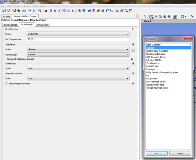
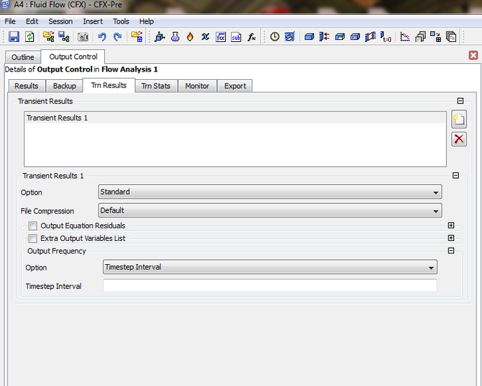
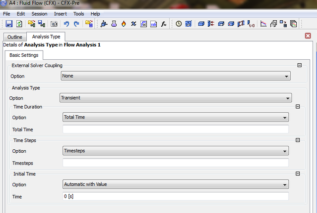
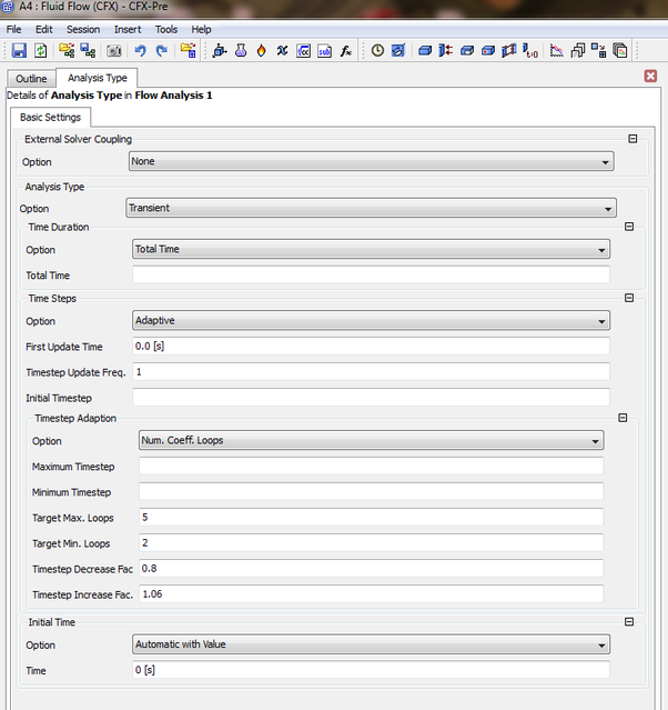
The following image shows an unsteady case with the available models to select from
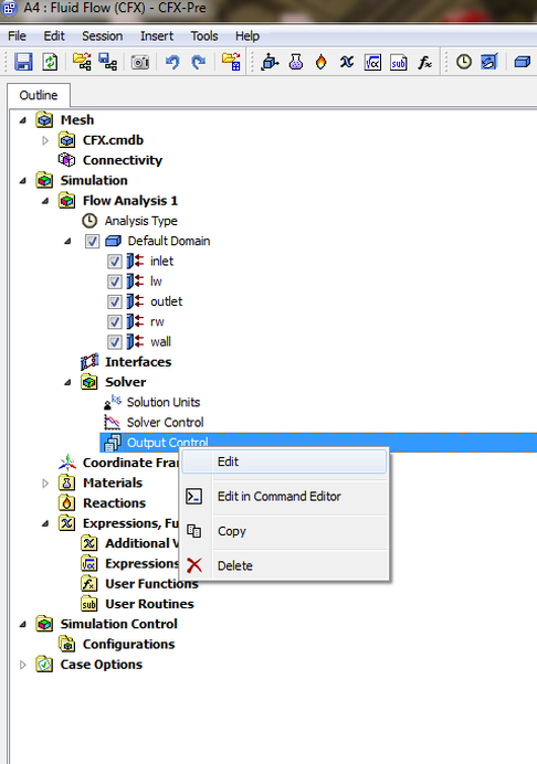
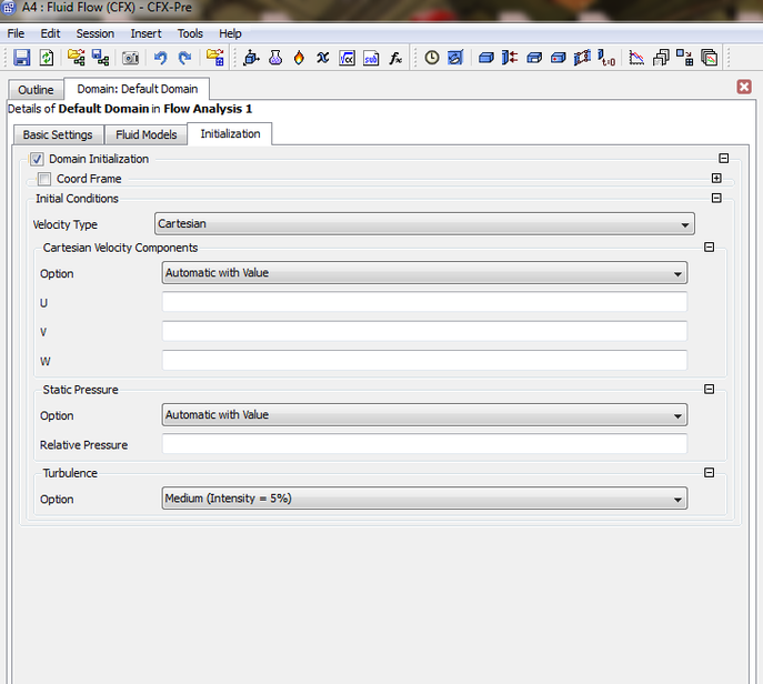
The user will need before starting to run a simulation to specify the save frequency during the writing up of the generated data in addition to specifying the initial conditions:
You will need to input the required time intervial
You will need to apply the initial conditions for the simulation or it will crash after starting your calculation.
Recommended Power Point Presentation Link:
http://www.google.co.uk/url?sa=t&rct=j&q=&esrc=s&source=web&cd=5&cad=rja&ved=0CFwQFjAE&url=http%3A%2F%2Fwww.petrodanesh.ir%2FVirtual%2520Education%2FMechanics%2FANSYS-CFX%2FLectures%2FCFX12_08_Transient.ppt&ei=XKu9UvacJYqRhQfSj4HYDg&usg=AFQjCNGY3H0hzay8WYdSkAaPe9suu9qyWA&sig2=6yiV1CtHyVhcyREj2mUZjQ
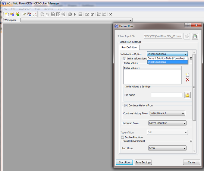
Initialization
You need to be careful and delete previous files if not then this can cause wrong data to be generated .
Steady Simulations
As an initial option of building a numerical model is to run it in a steady mode and that is for
1- To check that the selected grid density is enough to capture the required flow patterns.
2- To check that the produced results mimic experimental results.
3-.............................
4-.................
1- To check that the selected grid density is enough to capture the required flow patterns.
2- To check that the produced results mimic experimental results.
3-.............................
4-.................
Example
For a user of ANSYS CFX the first question comes to mind where will this be written and where will it be feed to ANSYS CFX, this will added soon.
Then comes
In the CCL example that follows, the solver starts with an internally calculated timescale multiplied by the Timescale Factor of 0.75. The internally calculated timescale is updated every 7 iterations, but is not permitted to exceed the Maximum Timescale of 5 [s]. The timescale is updated every 7 iterations for a total number of 12 updates. After this period, the timescale increases every iteration by a factor of 1.3 until it reaches the Maximum Timescale.
SOLVER CONTROL:
CONVERGENCE CONTROL:
Maximum Number of Iterations = 150
Timescale Control = Auto Timescale
Timescale Factor = 0.75
Number of Timescale Updates = 12
Timescale Update Frequency = 7
Maximum Timescale = 5 [s]
Timescale Ramping Factor = 1.3
END
END
CONVERGENCE CONTROL:
Maximum Number of Iterations = 150
Timescale Control = Auto Timescale
Timescale Factor = 0.75
Number of Timescale Updates = 12
Timescale Update Frequency = 7
Maximum Timescale = 5 [s]
Timescale Ramping Factor = 1.3
END
END
Static Time Stepping
This is used to study for a single process.
Controlling the Timescale for Each Equation
The problem.......................
Solid Time Scale Factor
This factor by default is 1 but when the researcher is working on a case of moving blades then more detail needs to know about the factor because it wouldn't be one, the researcher is adviced to have a look through the ANSYS CFX manual.
Time Scale Control
Under construction.
Maximum Timescale
The Maximum Timescale can be used to bound the internally-calculated time scale. The ANSYS CFX-Solver uses the smaller of the internally calculated time scale and the user maximum value.
Time Scale Factor
The Timescale Factor option, set automatically to a default value of 1, can be used to multiply the Auto Timescale value calculated by the solver.
Advection Time Scale
Local Time Scale Factor
Average Scale Information
Under Construction.
Physical Time Scale
Physical time scale in definition is a pretending time step, definitely not the real time.The Physical Timescale option allows a fixed time scale to be used for the selected equations over the entire flow domain. In most cases, there are two situations in which you would use a physical time scale:
1- To give sufficient relaxation to the none linear terms of the equation so that a converged steady-state solution can be achieved.
2- To evolve the solution through time in order to provide transient information about a time-dependent simulation.
For advection dominated flows (meaning of adviction dominated flows is where the transfer of a property of the atmosphere, such as heat, cold, or humidity, by the horizontal movement of an air mass), the physical time scale should be some fraction of a length scale divided by a velocity scale. A good approximation is the Dynamical Time for the flow. This is the time taken for a point in the flow to make its way through the fluid domain
Where L is the length scale and U is the velocity.
Length Scale Option
Unless otherwise noted, all content on this site is @Copyright by Ahmed Al Makky 2012-2014 - http://cfd2012.com
