Studying Fuel Sprays
Introduction
The environment has been a major issue on the news because it’s something that can’t be ignored any more why? The answer is why is there so many hurricanes, Al Neno, melting of ice caps in the north and south poles, winters are warmer than before ,hotter summers ,flooding and famines. Environmental friendly technology is a reality and an important demand which is telling us humans to become more responsibly aware and less selfish.
The coming factors are affecting the whole world:
1- Depletion of fuel sources.
2-Security of supply issues ,recently the Russian gas pipe line crises with European
countries ,the instability of the middle east region .
3- The Kyoto protocol and Co2 targets set for countries to achieve.
4-Getting more efficient combustion process with less Co2 ,Co,Soot,Nox,Sox emissions because these gases have devastating environmental effects like acid rain on forests and buildings ,for large inhabited cities like the photo chemical Smog covering Los Angles and kula Lumpour.
5- Chinese and Indian growing demand for fuel to back up there increasing growth rates.
6-The rise of oil prises were it got over $70 a barrel at one stage in the last couple of years, this has made expensive technologies to be an attractive alternative to governments due the decreasing price gap between classical fuels and alternatives.
These factors have contributed in the need of companies and governments in investing time and money in finding and introducing new technologies to be used all over the world, Japanese manufactures took the lead and were one of the leading countries introducing fuel economic models during the seventies such as Nissan sunny B110,B210series and later on Mitsubishi motors’ introduced GDI technology into car engines to also make them a more attractable choice for fuel economy and high efficiency. This has made countries to look for alternative fuels which are cheap clean and easy to burn. But to our disappointment in life there is nothing ideal, but what we can do is try to make it as ideal as possible, as an example it might be clean but it is only found on the other side of the planet. In the near future(and this has started in a couple of countries for example GMC company in America, were it has models that run on 85% ethanol and 15% gasoline) car engines are going to be designed to work on several kinds of fuels on a separate base or a mixed base and due to the introduction of hybrid technology such as fuel cells , cars will be alternating during trips and switching from electrical mode to fuel burning engine mode. This will force manufactures to use special types of atomizers and variable pressure pumps at different output pressures to suite the atomization mode required by the driver (Sports mode or economic mode). That will also lead manufacturers in using special types of piston heads that will be compatible to use on several types of fuels and at the same time giving out the best mechanical output efficiency.
Fuel Atomization Lab
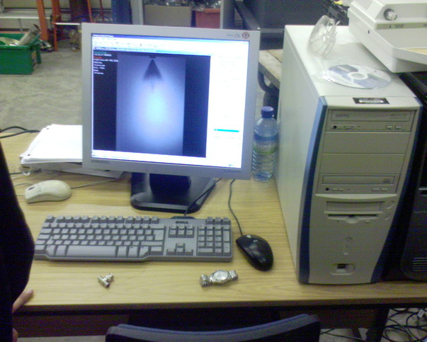
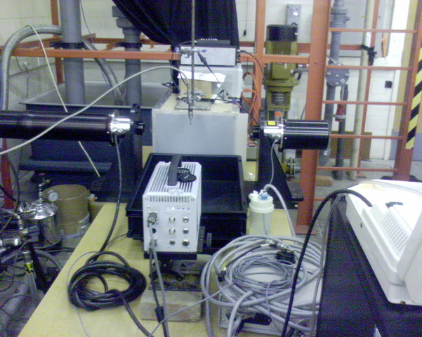
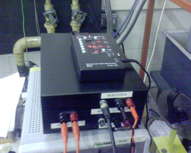
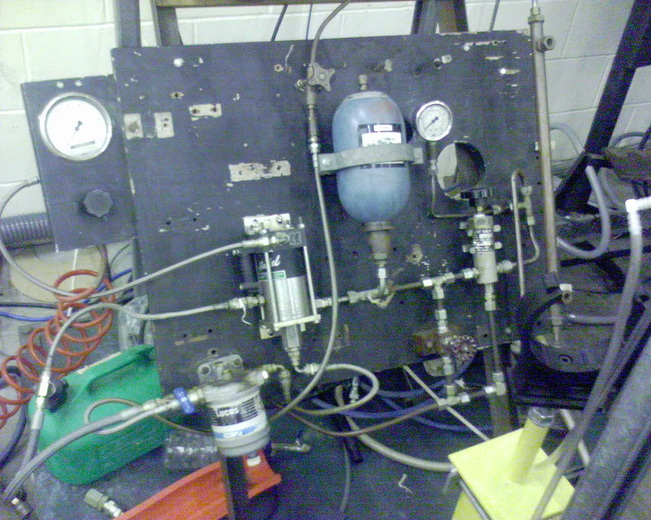
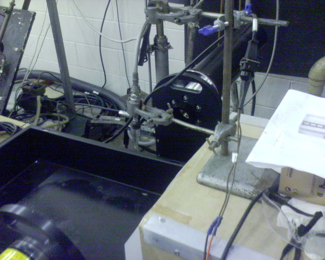
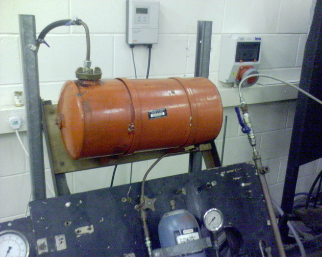
The next set of pictures provided in the album gives a descriptive description of the experimental setup, the high pressure jet atomization is shown at one time frame is shown, anther frame is shown to the low pressure jet atomization is also shown. The computer desktop is shown with the used software. Experience in the fuel atomization lab. The high frame rate camera used is also shown. Fuel tank is shown in an orange colour fro it fuel is passed to the high/low pressure injector. A Laser beam is also used to analyse the particle distribution of atomized fuel droplets. The liquid collection sink is also shown. The two pressure gauges used are to read how much pressure difference was applied to the injector. Air pressure is used in the process.
Insitec RTSizer for Windows ASCII data - A:\GDI_spray_ANALYSIS.txt
Start Date-Time = X Feb 20XX XX:XX:XX.XXXX
Stop Date-Time = X Feb 20XX XX:XX:XX.XXXX
Material : smoke Lot : 2 Experiment : 0
Notes :
Status = Valid
Data Type
Volume
Error Code = 0
****************************************************************************************
Measurement Assumptions
Calibration : (ST45AIAC.CAL, STAEUNIT.IMG, STUNITY.RSP)
Lens = 450
Media Refractive Index = 1.00 + 0.00i
Particulate Refractive Index = 1.50 + 0.50i
Path Length = 12.00 (mm)
Particulate Density = 1.00 (gm/cc)
Mesh Factor = 1.00
Laser Wavelength = 670.0 (nm)
****************************************************************************************
Standard Values
T = 74.48%
Cv = 21.85 (LWC)
Span = 2.24
Specific Surface Area (m^2/cc) = 2.001068
Dv(10) = 1.26 (µm)
Dv(50) = 4.78 (µm)
Dv(90) = 11.99 (µm)
D[3][2] = 3.00 (µm)
D[4][3] = 5.83 (µm)
****************************************************************************************
Scattering Results
Ring Scattering Raw Scat Background
0 1311.00 1311.00 1760.31
1 0.00 0.00 1.00
2 0.00 35.50 42.31
3 0.00 53.75 49.31
4 3.13 17.75 21.44
5 2.88 17.94 17.44
6 1.88 9.38 11.06
7 0.75 6.69 7.56
8 0.69 5.00 6.13
9 0.88 4.50 4.19
10 0.94 4.00 4.31
11 1.19 2.88 2.13
12 1.50 3.88 2.75
13 2.38 3.19 1.81
14 3.69 6.50 2.25
15 4.75 5.94 2.19
16 5.38 9.38 3.31
17 6.63 5.38 0.00
18 9.75 16.44 6.69
19 14.38 17.19 3.88
20 13.38 26.00 4.88
21 12.81 679.88 1534.63
22 27.44 50.94 19.19
23 47.63 60.38 10.06
24 65.56 75.94 7.69
25 87.13 98.00 8.75
26 115.13 126.00 5.50
27 150.38 163.00 3.31
28 194.06 210.50 5.00
29 246.44 268.06 3.19
30 307.38 332.00 3.56
31 372.88 412.50 2.38
****************************************************************************************
Size Results
% Volume % Number Dupper (um) Dlower (um)
0.0000 0.0000 0.1166 0.1000
0.0000 0.0000 0.1359 0.1166
0.0000 0.0000 0.1585 0.1359
0.0000 0.0000 0.1848 0.1585
0.0000 0.0000 0.2154 0.1848
0.0000 0.0000 0.2512 0.2154
0.0000 0.0000 0.2929 0.2512
0.0000 0.0000 0.3415 0.2929
0.0000 0.0000 0.3981 0.3415
0.0000 0.0000 0.4642 0.3981
0.0000 0.0000 0.5412 0.4642
0.0004 0.0098 0.6310 0.5412
0.0176 0.2867 0.7356 0.6310
0.0201 0.2066 0.8577 0.7356
0.0227 0.1474 1.0000 0.8577
0.0255 0.1046 1.1659 1.0000
0.0286 0.0739 1.3594 1.1659
0.0319 0.0521 1.5849 1.3594
0.0356 0.0367 1.8478 1.5849
0.0396 0.0257 2.1544 1.8478
0.0439 0.0180 2.5119 2.1544
0.0484 0.0125 2.9286 2.5119
0.0532 0.0087 3.4145 2.9286
0.0580 0.0060 3.9811 3.4145
0.0626 0.0041 4.6416 3.9811
0.0668 0.0027 5.4117 4.6416
0.0700 0.0018 6.3096 5.4117
0.0716 0.0012 7.3564 6.3096
0.0707 0.0007 8.5770 7.3564
0.0666 0.0004 10.0000 8.5770
0.0585 0.0002 11.6591 10.0000
0.0466 0.0001 13.5936 11.6591
0.0321 0.0001 15.8489 13.5936
0.0181 0.0000 18.4785 15.8489
0.0079 0.0000 21.5443 18.4785
0.0025 0.0000 25.1189 21.5443
0.0006 0.0000 29.2864 25.1189
0.0001 0.0000 34.1455 29.2864
0.0000 0.0000 39.8107 34.1455
0.0000 0.0000 46.4159 39.8107
0.0000 0.0000 54.1170 46.4159
0.0000 0.0000 63.0957 54.1170
0.0000 0.0000 73.5642 63.0957
0.0000 0.0000 85.7696 73.5642
0.0000 0.0000 100.0000 85.7696
0.0000 0.0000 116.5914 100.0000
0.0000 0.0000 135.9356 116.5914
0.0000 0.0000 158.4893 135.9356
0.0000 0.0000 184.7850 158.4893
0.0000 0.0000 215.4435 184.7850
0.0000 0.0000 251.1886 215.4435
0.0000 0.0000 292.8645 251.1886
0.0000 0.0000 341.4549 292.8645
0.0000 0.0000 398.1072 341.4549
0.0000 0.0000 464.1589 398.1072
0.0000 0.0000 541.1695 464.1589
0.0000 0.0000 630.9573 541.1695
0.0000 0.0000 735.6423 630.9573
0.0000 0.0000 857.6959 735.6423
0.0000 0.0000 1000.0000 857.6959
****************************************************************************************
Process Control Variable Results
Value (Avg) Std Dev Max Min Variable Title - [Correction Equation]
1.259 0.000 0.000 0.000 Dv(10.0) (µm) - [Xc = X]
4.780 0.000 0.000 0.000 Dv(50.0) (µm) - [Xc = X]
11.990 0.000 0.000 0.000 Dv(90.0) (µm) - [Xc = X]
74.475 0.000 0.000 0.000 Transmission (%) - [Xc = X]
5.829 0.000 0.000 0.000 D[4][3] (µm) - [Xc = X]
4.813 0.000 0.000 0.000 Dv(50.0) (µm) : Avg - [Xc = X]
*********************************************End Of File*******************************************
Will upload some samples of high and low pressure spray histograms, the following one is for high pressure:
Lasers have been mainly used to characterize the two-dimensional fuel vapour concentration inside the cylinder of a all types of valve spark ignition engines equipped with high and low-pressure injectors. The effects of injection timing, on the test bench charge motion and injector tip layout have been quantified. The flexibility in nozzle design of swirl-hole injectors has proven to be a powerful tool in terms of matching overall spray cone angle and number of holes to specific engine configurations. Injection timing was found to control spray impingement on the piston and cylinder wall, thus contributing to quick and efficient fuel evaporation. It was confirmed that in-cylinder charge motion plays a major role in engine’s stable operation by assisting in the transportation of the air-fuel mixture towards the ignition locations (i.e. spark-plugs) in the way of a uniformly distributed charge or by preserving stratification of the charge depending on operating mode of the engine.
The picture below shows the test rig used to control what kind pressure pulses that the researcher wants to produce, notcie fixed accumelator and the prssure selonode fixed on the mid section.
The following picture shows the tested spray tip fixed on the test rig, different types of nozzels where tested.
The picture below shows the fuel tank used to store the required fuel for conducting atmoization tests.
Some important values in order to get the feel of the numbers worked on:
Mean Droplet Diameter 50 micron
Spray occurs at 3 bar
Volumetric flow rates 0.00000065 m^3/s or 19,5 CC/min
Mass flow rates 7.96E-12 kg/s
Densities:
Water 998 kg/m^3
Kerosene 810 kg/m^3
Diesel 800 kg/m^3
Gasoline 770 kg/m^3
Mean Droplet Diameter 50 micron
Spray occurs at 3 bar
Volumetric flow rates 0.00000065 m^3/s or 19,5 CC/min
Mass flow rates 7.96E-12 kg/s
Densities:
Water 998 kg/m^3
Kerosene 810 kg/m^3
Diesel 800 kg/m^3
Gasoline 770 kg/m^3
The following set of data can form input paramters for a simulation for a case of CFD modeling of Heavy Fuel Oil (HFO) spray combustion
Gasoil temp = 44 C
Mean diameter = 81 micro-meter
LHV = 43.005 MJ/kg
Spray angle = 89 DRG
========================
HFO temp = 100 C
Mean diameter = 91 micro-meter
LHV= 40.915 MJ/kg
Spray angle = 79 DRG
========================
There is no significant difference between injection patterns.
Mean diameter = 81 micro-meter
LHV = 43.005 MJ/kg
Spray angle = 89 DRG
========================
HFO temp = 100 C
Mean diameter = 91 micro-meter
LHV= 40.915 MJ/kg
Spray angle = 79 DRG
========================
There is no significant difference between injection patterns.
Unless otherwise noted, all content on this site is @Copyright by Ahmed Al Makky 2012-2018 - http://cfd2012.com
