A Tutorial on Solving ODEs using MATLAB
Example Using TDMA
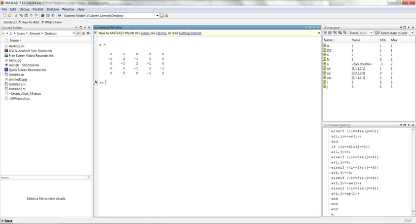
Using TDMA, deriving the TDMA method using MATLAB, solving the problem in a step by step method:
%Forming TDMA matrix
clc
clear
N=5;
A=1;
K=1;
DX=1;
for i=1:N;
aw(i)=(K*A)/DX;
ae(i)=(K*A)/DX;
ap(i)=aw(i)+ae(i);
end
for i=1:N;
for j=1:N;
if ((i==1)&(j==1))
a(i,j)=ap(i);
elseif ((i==1)&(j==2))
a(i,j)=-ae(i);
elseif ((i==1)&(j>2))
a(i,j)=0;
end
if ((i==2)&(j==1))
a(i,j)=-ae(i);
elseif ((i==2)&(j==2))
a(i,j)=ap(i);
elseif ((i==2)&(j==3))
a(i,j)=-aw(i);
elseif ((i==2)&(j>3))
a(i,j)=0;
end
if ((i==3)&(j==1))
a(i,j)=0;
elseif ((i==3)&(j==2))
a(i,j)=-ae(i);
elseif ((i==3)&(j==3))
a(i,j)=ap(i);
elseif ((i==3)&(j==4))
a(i,j)=-aw(i);
elseif ((i==3)&(j>4))
a(i,j)=0;
end
if ((i==4)&(j==1))
a(i,j)=0;
elseif ((i==4)&(j==2))
a(i,j)=0;
elseif ((i==4)&(j==3))
a(i,j)=-ae(i);
elseif ((i==4)&(j==4))
a(i,j)=ap(i);
elseif ((i==4)&(j==5))
a(i,j)=-aw(i);
end
if ((i==5)&(j==1))
a(i,j)=0;
elseif ((i==5)&(j==2))
a(i,j)=0;
elseif ((i==5)&(j==3))
a(i,j)=-0;
elseif ((i==5)&(j==4))
a(i,j)=-aw(i);
elseif ((i==5)&(j==5))
a(i,j)=ap(i);
end
end
end
a
b-The provided code is a TDMA function. This following code constructs the diagonal matrix in a different method.
function x = TDMAsolver(a,b,c,d)
%a, b, c, and d are the column vectors for the compressed tridiagonal matrix
n = length(b);
% n is the number of rows
% Modify the first-row coefficients
c(1) = c(1) / b(1);
% Division by zero risk.
d(1) = d(1) / b(1);
% Division by zero would imply a singular matrix.
for i = 2:n id = 1 / (b(i) - c(i-1) * a(i));
% Division by zero risk.
c(i) = c(i)* id;
% Last value calculated is redundant.
d(i) = (d(i) - d(i-1) * a(i)) * id;
end
% Now back substitute.
x(n) = d(n);
for i = n-1:-1:1
x(i) = d(i) - c(i) * x(i + 1);
end
end
Other Proposed Methods
Some provided functions in MATLAB used to solve a set of algebraic equations
1-Cholesky Factorization. Example R=chol(A).
2-LU: Factorization.Example [L,U]=lu(A)
3-QR:Factorization.
1-Cholesky Factorization. Example R=chol(A).
2-LU: Factorization.Example [L,U]=lu(A)
3-QR:Factorization.
Example Coding the Standard Deviation Method for a Set of 1D Velocity and then comparing the Output with the Built in Function in MATLAB
clc
clear
N=10;
for i=1:N+1
mb=randn(1,1);
if mb>1
V(i)=-rand(1,1);
else
V(i)=rand(1,1);
end
end
%Finding the standard deviation direct;y from matlab
s=std(V(:));
%Programing the standard deviation
jh=size(V(:));
mu=sum(V(:))/jh(1);
for i=1:N+1
vl(i)=(V(i)-mu)^2;
end
ss=(sum(vl(:))/(jh(1)-1))^0.5;
%Standard Deviation finished code
%Next finding the Skewness
for i=1:N+1
VVV(i)=(V(i))^3;
end
VV=mean(sum(VVV(:)));
skewness(V(:));
SKEWN=VV/(s)^3;
%Finding the variance
f=var(V(:));
Example Conducting a study on a Heat Transfer Case in a Solid:
Finite Volume 1D Steady Heat Diffusion Studied Case, the code uses TDMA.
clc
clear
K=100;
A=0.01;
TA=100;
TB=500;
L=1;
N=500;
DX=L/N;
for I=1:N
X(I)=I*DX;
end
for I=1:N;
if (I==1)
SU(I)=(2*K*A*TA)/DX;
SP(I)=(-2*K*A)/DX;
AW(I)=0; AE(I)=(K*A)/DX;
AP(I)=AE(I)+AW(I)-SP(I);
AA(I)=-1*AW(I);
BB(I)=AP(I);
CC(I)=-1*AE(I);
DD(I)=SU(I);
elseif (I==N)
SU(I)=(2*K*A*TB)/DX;
SP(I)=(-2*K*A)/DX;
AW(I)=(K*A)/DX;
AE(I)=0;
AP(I)=AE(I)+AW(I)-SP(I);
AA(I)=-1*AW(I);
BB(I)=AP(I);
CC(I)=-1*AE(I);
DD(I)=SU(I);
elseif ((I~=1)|(I~=N))
SU(I)=0;
SP(I)=0;
AW(I)=(K*A)/DX;
AE(I)=(K*A)/DX;
AP(I)=AE(I)+AW(I);
AA(I)=-1*AW(I);
BB(I)=AP(I);
CC(I)=-1*AE(I);
DD(I)=0;
end
end
CC(1)=CC(1)/BB(1);
DD(1)=DD(1)/BB(1);
for I=2:N;
ID(I)=1/(BB(I)-CC(I-1)*AA(I));
CC(I)=CC(I)*ID(I);
DD(I)=(DD(I)-DD(I-1)*AA(I))*ID(I);
end
T(N)=DD(N);
I=N;
for J=1:N-1;
I=I-1;
T(I)=DD(I)-CC(I)*T(I+1);
end
%CHECKING OUTPUT
% AW' % AE' % SU' % SP' % AP'
% T' plot(X,T);
grid on;
xlabel('X');
Ylabel('T');
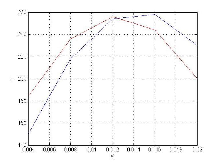
Finite Volume 1D Steady Heat Diffusion with Heat Source,the code uses TDMA
clc
clear
K=0.5;
A=1;
TA=100;
TB=200;
L=0.02;
N=5;
DX=L/N;
q=1000000;
for I=1:N;
X(I)=I*DX;
end
for I=1:N;
if (I==1)
SU(I)=(2*K*A*TA)/DX+q*A*DX;
SP(I)=(-2*K*A)/DX;
AW(I)=0;
AE(I)=(K*A)/DX;
AP(I)=AE(I)+AW(I)-SP(I);
AA(I)=-1*AW(I);
BB(I)=AP(I);
CC(I)=-1*AE(I);
DD(I)=SU(I);
elseif (I==N) SU(I)=(2*K*A*TB)/DX+q*A*DX;
SP(I)=(-2*K*A)/DX;
AW(I)=(K*A)/DX;
AE(I)=0;
AP(I)=AE(I)+AW(I)-SP(I);
AA(I)=-1*AW(I);
BB(I)=AP(I);
CC(I)=-1*AE(I);
DD(I)=SU(I);
elseif ((I~=1)|(I~=N))
SU(I)=+q*A*DX;
SP(I)=0;
AW(I)=(K*A)/DX;
AE(I)=(K*A)/DX;
AP(I)=AE(I)+AW(I);
AA(I)=-1*AW(I);
BB(I)=AP(I);
CC(I)=-1*AE(I);
DD(I)=SU(I);
end
end
CC(1)=CC(1)/BB(1);
DD(1)=DD(1)/BB(1);
for I=2:N;
ID(I)=1/(BB(I)-CC(I-1)*AA(I));
CC(I)=CC(I)*ID(I);
DD(I)=(DD(I)-DD(I-1)*AA(I))*ID(I);
end
T(N)=DD(N);
I=N;
for J=1:N-1;
I=I-1;
T(I)=DD(I)-CC(I)*T(I+1);
end
%CHECKING OUTPUT % AW' %AE' %SU' %SP' %AP' %T' % EXACT solution
for i=1:N;
TT(i)=((TB-TA)/L)*X(i)+(0.5*q)*((L-X(i))*X(i))/K+TA;
end
plot(X,T);
grid on;
xlabel('X');
Ylabel('T');
hold on;
plot(X,TT,'-r')
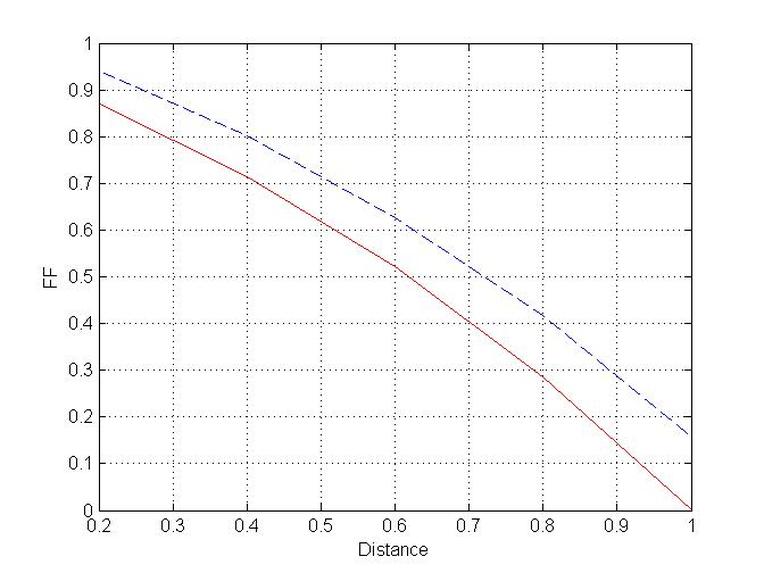
Finite Volume 1D Steady Convection Diffusion ,the code uses TDMA
clc
clear
N=5;
FFA=1;
FFB=0;
DX=0.2;
for I=1:N;
X(I)=I*DX;
if (I==1)
DENSITYw(I)=0;
DENSITYe(I)=1;
Uw(I)=0;
Ue(I)=0.1;
Rw(I)=0;
Re(I)=0.1;
DELTAXWP(I)=0.2;
DELTAXPE(I)=0.2;
Fw(I)=DENSITYw(I)*Uw(I);
Fe(I)=DENSITYe(I)*Ue(I);
Dw(I)=Rw(I)/DELTAXWP(I);
De(I)=Re(I)/DELTAXPE(I);
AW(I)=0;
AE(I)=De(I)-0.5*Fe(I);
SP(I)=-(2*De(I)+Fe(I));
AP(I)=AW(I)+AE(I)-SP(I);
Su(I)=(2*De(I)+Fe(I))*FFA;
AA(I)=-1*AW(I);
BB(I)=AP(I);
CC(I)=-1*AE(I);
DD(I)=Su(I);
elseif (I==N) DENSITYw(I)=1;
DENSITYe(I)=0;
Uw(I)=0.1;
Ue(I)=0;
Rw(I)=0.1;
Re(I)=0;
DELTAXWP(I)=0.2;
DELTAXPE(I)=0.2;
Fw(I)=DENSITYw(I)*Uw(I);
Fe(I)=DENSITYe(I)*Ue(I);
Dw(I)=Rw(I)/DELTAXWP(I);
De(I)=Re(I)/DELTAXPE(I);
AW(I)=Dw(I)+0.5*Fw(I);
AE(I)=0;
SP(I)=-(2*Dw(I)-Fw(I));
AP(I)=AW(I)+AE(I)-SP(I);
Su(I)=(2*Dw(I)+Fw(I))*FFB; AA(I)=-1*AW(I); BB(I)=AP(I);
CC(I)=-1*AE(I); DD(I)=Su(I); elseif ((I~=I)|(I~=N)) DENSITYw(I)=1; DENSITYe(I)=1; Uw(I)=0.1; Ue(I)=0.1; Rw(I)=0.1; Re(I)=0.1; DELTAXWP(I)=0.2; DELTAXPE(I)=0.2; Fw(I)=DENSITYw(I)*Uw(I); Fe(I)=DENSITYe(I)*Ue(I); Dw(I)=Rw(I)/DELTAXWP(I); De(I)=Re(I)/DELTAXPE(I); AW(I)=Dw(I)+0.5*Fw(I); AE(I)=De(I)-0.5*Fe(I); AP(I)=AW(I)+AE(I)+(Fe(I)-Fw(I)); SP(I)=0; Su(I)=0; AA(I)=-1*AW(I);
BB(I)=AP(I); CC(I)=-1*AE(I);
DD(I)=Su(I);
end
end
%checking output
% AW' % AE' % Su' % SP' % AP'
CC(1)=CC(1)/BB(1);
DD(1)=DD(1)/BB(1);
for I=2:N;
ID(I)=1/(BB(I)-CC(I-1)*AA(I));
CC(I)=CC(I)*ID(I);
DD(I)=(DD(I)-DD(I-1)*AA(I))*ID(I);
end
FF(N)=DD(N);
I=N;
for J=1:N-1; I=I-1;
FF(I)=DD(I)-CC(I)*FF(I+1);
end
for I=1:N;
t(I)=I*DX;
FFF(I)=(2.7183-exp(t(I)))/1.7183;
end
%THIS IS JUST TO VALIDATE OUTPUT
% PP=[1.55 -0.45 0 0 0; -0.55 1.0 -0.45 0 0; 0 -0.55 1.0 -0.45 0; 0 0 -0.55 1.0 -0.45; 0 0 0 -0.55 1.45];
% PPP=[1.1 0 0 0 0]';
% PPPP=(PP^(-1))*(PPP);
%checking output
% ID= ID'
% CC=CC'
% BB=BB'
% DD=DD'
% AA=AA'
% FF=FF'
plot(X,FF,'--B')
grid on;
xlabel('Distance')
ylabel('FF')
hold on
plot(X,FFF,'-r')
%THIS IS JUST TO VALIDATE OUTPUT
% hold on
% plot(X,PPPP,'--r')
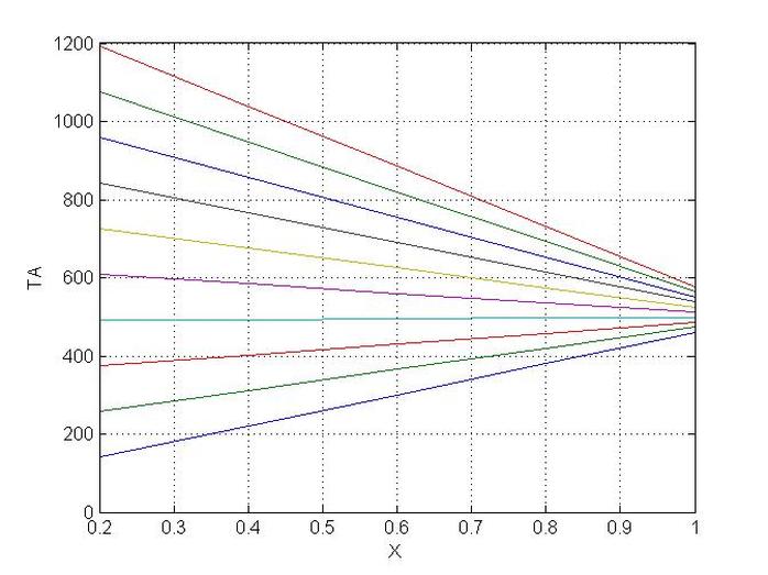
Finite Volume 1D Heat Diffusion Studied Case, that offers the option to show different heat profiles for a changing temperature boundary the code uses TDMA.
clc
clear
K=100;
A=0.01;
TIME=1;
TIMEA=1;
TIMEB=1;
TA(TIMEA)=100;
TB(TIMEB)=500;
L=1; N=5;
DX=L/N;
for I=1:N
X(I)=I*DX;
end
TIMEA=0;
for TIME=1:10; TIMEA=TIMEA+1;
TA(TIMEA+1)=TA(TIMEA)+130;
for I=1:N;
if (I==1) SU(I,TIME)=(2*K*A*TA(TIMEA))/DX;
SP(I,TIME)=(-2*K*A)/DX; AW(I,TIME)=0;
AE(I,TIME)=(K*A)/DX; AP(I,TIME)=AE(I,TIME)+AW(I,TIME)-SP(I,TIME);
AA(I)=-1*AW(I,TIME); BB(I)=AP(I,TIME);
CC(I)=-1*AE(I,TIME); DD(I)=SU(I,TIME);
elseif (I==N) SU(I,TIME)=(2*K*A*TB(TIMEB))/DX;
SP(I,TIME)=(-2*K*A)/DX; AW(I,TIME)=(K*A)/DX;
AE(I,TIME)=0; AP(I,TIME)=AE(I,TIME)+AW(I,TIME)-SP(I,TIME);
AA(I)=-1*AW(I,TIME);
BB(I)=AP(I,TIME);
CC(I)=-1*AE(I,TIME);
DD(I)=SU(I,TIME);
elseif ((I~=1)|(I~=N))
SU(I,TIME)=0; SP(I,TIME)=0;
AW(I,TIME)=(K*A)/DX;
AE(I,TIME)=(K*A)/DX;
AP(I,TIME)=AE(I,TIME)+AW(I,TIME);
AA(I)=-1*AW(I,TIME);
BB(I)=AP(I,TIME);
CC(I)=-1*AE(I,TIME);
DD(I)=0; end
end
CC(1)=CC(1)/BB(1);
DD(1)=DD(1)/BB(1);
for I=2:N;
ID(I)=1/(BB(I)-CC(I-1)*AA(I));
CC(I)=CC(I)*ID(I);
DD(I)=(DD(I)-DD(I-1)*AA(I))*ID(I);
end
T(N,TIME)=DD(N);
I=N;
for J=1:N-1;
I=I-1;
T(I,TIME)=DD(I)-CC(I)*T(I+1,TIME);
end
%CHECKING OUTPUT
% AW'
% AE'
% SU'
% SP'
% AP'
% T'
plot(X,T);
grid on;
xlabel('X');
Ylabel('TA');
hold on
end
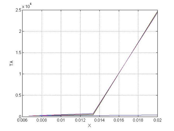
Finite Volume 1D Unsteady Heat Diffusion Studied Case Using Crank Nicholson, the Code Uses TDMA.
NOTE: The Method will be Validated Soon.
clc
clear
K=10;
A=0.01;
TIME=1;
TIMEA=1;
TIMEB=1;
TA(TIMEA)=200;
TB(TIMEB)=-100*TIMEB+500;
L=0.02;
N=3;
DX=L/N;
THETA=0.5;
HEAT_CAPACITY=1000000;
DENSITY=10;
for I=1:N
X(I)=I*DX;
end
%-------------------------------------------------------------------------- %-INITILIZATION------------------------------------------------------------
TIME=1;
for I=1:N;
if (I==1)
SU(I,TIME)=(2*K*A*TA(TIMEA))/DX;
SP(I,TIME)=(-2*K*A)/DX;
AW(I,TIME)=0;
AE(I,TIME)=(K*A)/DX;
AP(I,TIME)=AE(I,TIME)+AW(I,TIME)-SP(I,TIME);
AA(I)=-1*AW(I,TIME);
BB(I)=AP(I,TIME);
CC(I)=-1*AE(I,TIME);
DD(I)=SU(I,TIME);
elseif (I==N)
SU(I,TIME)=(2*K*A*TB(TIMEB))/DX;
SP(I,TIME)=(-2*K*A)/DX;
AW(I,TIME)=(K*A)/DX; AE(I,TIME)=0;
AP(I,TIME)=AE(I,TIME)+AW(I,TIME)-SP(I,TIME);
AA(I)=-1*AW(I,TIME);
BB(I)=AP(I,TIME);
CC(I)=-1*AE(I,TIME);
DD(I)=SU(I,TIME);
elseif ((I~=1)|(I~=N))
SU(I,TIME)=0;
SP(I,TIME)=0;
AW(I,TIME)=(K*A)/DX;
AE(I,TIME)=(K*A)/DX;
AP(I,TIME)=AE(I,TIME)+AW(I,TIME);
AA(I)=-1*AW(I,TIME);
BB(I)=AP(I,TIME);
CC(I)=-1*AE(I,TIME);
DD(I)=0;
end
end
CC(1)=CC(1)/BB(1);
DD(1)=DD(1)/BB(1);
for I=2:N;
ID(I)=1/(BB(I)-CC(I-1)*AA(I));
CC(I)=CC(I)*ID(I);
DD(I)=(DD(I)-DD(I-1)*AA(I))*ID(I);
end
T(N,TIME)=DD(N);
I=N;
for J=1:N-1;
I=I-1;
T(I,TIME)=DD(I)-CC(I)*T(I+1,TIME);
end
%CHECKING OUTPUT
% AW'
% AE'
% SU'
% SP'
% AP'
% T'
plot(X,T);
grid on;
xlabel('X');
Ylabel('TA');
hold on
%-------------------------------------------------------------------------- %-END_INITILIZATION--------------------------------------------------------
I=1;
TIME=1;
DELTA_TIME=((DX)^2)*(DENSITY*HEAT_CAPACITY)/(2*K);
%STARTING_TIME_STEPPING----------------------------------------------------
TIMEB=0
FINAL_TIME=4;
for TIME=1:FINAL_TIME;
TIMEB=TIMEB+1; TB(TIMEB)=-100*TIMEB+500;
for I=1:N;
if (I==1) SU(I,TIME+1)=(2*K*A*TA(TIMEA))/DX;
SP(I,TIME+1)=(-2*K*A)/DX; AW(I,TIME+1)=0;
AE(I,TIME+1)=(K*A)/DX;
AP0(I,TIME)=(DX*DENSITY*HEAT_CAPACITY)/DELTA_TIME; AP(I,TIME+1)=THETA*(AW(I,TIME+1)+AE(I,TIME+1))+AP0(I,TIME); AA(I)=-1*THETA*AW(I,TIME+1);
BB(I)=AP(I,TIME+1); CC(I)=-1*THETA*AE(I,TIME+1);
DD(I)=SU(I,TIME+1)+(1-THETA)*(T(I+1,TIME))+AP0(I,TIME)*T(I,TIME)-(1-THETA)*((AW(I,TIME+1))*T(I,TIME)+ (AE(I,TIME+1))*(T(I,TIME))); elseif (I==N)
SU(I,TIME+1)=(2*K*A*TB(TIMEB))/DX;
SP(I,TIME+1)=(-2*K*A)/DX; AW(I,TIME+1)=(K*A)/DX; AE(I,TIME+1)=0; AP0(I,TIME)=(DX*DENSITY*HEAT_CAPACITY)/DELTA_TIME;
AP(I,TIME+1)=THETA*(AW(I,TIME+1)+AE(I,TIME+1))+AP0(I,TIME);
AA(I)=-1*THETA*AW(I,TIME); BB(I)=AP(I,TIME);
CC(I)=-1*THETA*AE(I,TIME);
DD(I)=SU(I,TIME+1)+(1-THETA)*(T(I-1,TIME))+AP0(I,TIME)*T(I,TIME)-(1-THETA)*((AW(I,TIME+1))*T(I,TIME)+ (AE(I,TIME+1))*(T(I,TIME)));
elseif ((I~=1)|(I~=N))
SU(I,TIME+1)=0;
SP(I,TIME+1)=0;
AW(I,TIME+1)=(K*A)/DX;
AE(I,TIME+1)=(K*A)/DX;
AP0(I,TIME)=(DX*DENSITY*HEAT_CAPACITY)/DELTA_TIME; AP(I,TIME+1)=THETA*(AW(I,TIME+1)+AE(I,TIME+1))+AP0(I,TIME); AA(I)=-1*AW(I,TIME+1);
BB(I)=AP(I,TIME+1); CC(I)=-1*AE(I,TIME+1); DD(I)=(1-THETA)*(T(I+1,TIME)+T(I-1,TIME))+AP0(I,TIME)*T(I,TIME)-(1-THETA)*((AW(I,TIME+1))*T(I,TIME)+ (AE(I,TIME+1))*(T(I,TIME)));
end
end
CC(1)=CC(1)/BB(1);
DD(1)=DD(1)/BB(1);
for I=2:N;
ID(I)=1/(BB(I)-CC(I-1)*AA(I));
CC(I)=CC(I)*ID(I);
DD(I)=(DD(I)-DD(I-1)*AA(I))*ID(I);
end
T(N,TIME+1)=DD(N);
I=N;
for J=1:N-1;
I=I-1;
T(I,TIME+1)=DD(I)-CC(I)*T(I+1,TIME+1);
end
plot(X,T);
end
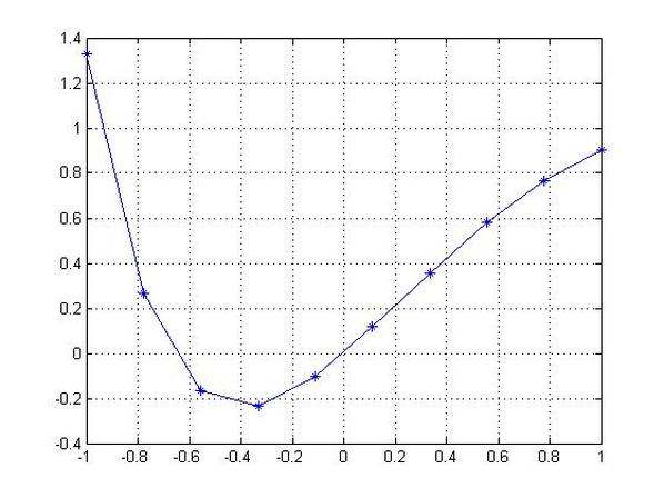
Using MATLAB Functions to Solve ODEs
clc
clear
eqn2= 'D3y+3*D2y+3*Dy+2*y=x^3';
init2= 'y(0)=0,Dy(0)=1,D2y(0)=1';
y=dsolve(eqn2,init2,'x')
x=linspace(-1,1,10);
z=eval(vectorize(y));
plot(x,z,'-*')
grid on
clear
eqn2= 'D3y+3*D2y+3*Dy+2*y=x^3';
init2= 'y(0)=0,Dy(0)=1,D2y(0)=1';
y=dsolve(eqn2,init2,'x')
x=linspace(-1,1,10);
z=eval(vectorize(y));
plot(x,z,'-*')
grid on
Unless otherwise noted, all content on this site is @Copyright by Ahmed Al Makky 2012-2013 - http://cfd2012.com