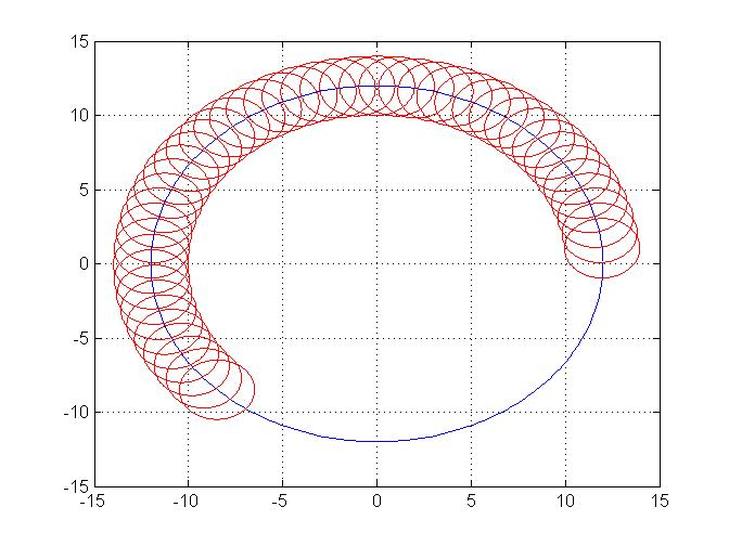
Restricting a Circle to Circular Path
clc
clear
N=360;
R=12;
r=2;
theta(1)=0;
for i=1:N;
theta(i+1)=theta(i)+1;
alpha(i)=(pi/180)*theta(i+1);
end
for i=1:N;
x0(i)=R*cos(alpha(i));
y0(i)=R*sin(alpha(i));
end
plot(x0,y0)
grid on
hold on
c=0;
for j=1:45;
c=c+5;
for i=1:N;
x(i)=r*cos(alpha(i))+x0(c);
y(i)=r*sin(alpha(i))+y0(c);
end
plot(x,y,'r')
hold on
end
Matrix Algebraic Operations
clc
clear
M=1;
N=5;
%One Dimensional Matrix
for i=1:M;
for j=1:N;
x(i,j)=randn(1,1);
end
end
%One Dimensional Matrix Transpose
for i=1:M;
for j=1:N;
xt(j,i)=x(i,j);
end
end
%Checking Output x xt for i=1:M; for j=1:N;
xxxt(j,i)=x(i,j)*xt(j,i);
end
end
xxt=sum(xxxt)
x*xt
clear
M=1;
N=5;
%One Dimensional Matrix
for i=1:M;
for j=1:N;
x(i,j)=randn(1,1);
end
end
%One Dimensional Matrix Transpose
for i=1:M;
for j=1:N;
xt(j,i)=x(i,j);
end
end
%Checking Output x xt for i=1:M; for j=1:N;
xxxt(j,i)=x(i,j)*xt(j,i);
end
end
xxt=sum(xxxt)
x*xt
Making Simulations
The following links are all related to making simulations.
http://www.mathworks.com/help/techdoc/creating_plots/f10-1460.html#brb6lra.
http://www.mathworks.com/help/techdoc/ref/feather.html
http://www.mathworks.com/help/techdoc/ref/comet3.html
http://www.mathworks.com/help/techdoc/ref/compass.html
http://www.mathworks.com/help/techdoc/ref/comet.html
http://www.mathworks.com/help/techdoc/ref/contourf.html
Working with barcharts in MATLAB.
LINK 1
LINK 2
LINK 3
Example Title
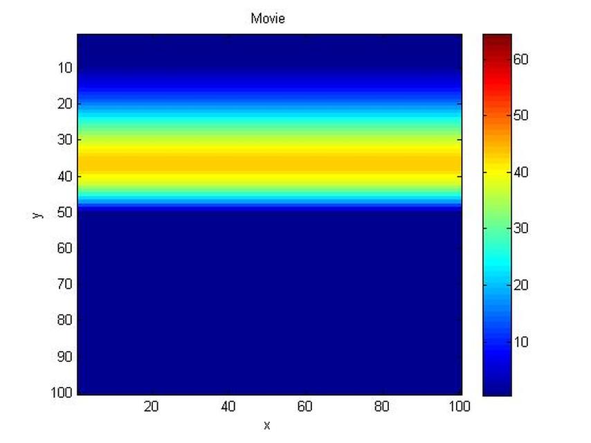
clc
clear
M=100;
N=100;
L=2;
x0=0;
xl=x0+L;
dx=L/M;
dy=L/N;
a=0.23;
tt=10;
for t=1:tt;
a=a+0.01;
for j=1:N;
for i=1:M;
x(i,j,t)=i*dx;
y(i,j,t)=j*dy;
yy(i,j,t)=1000*sin(pi*x(i,j))*(a*x(i,j))^2;
end
end
end
for t=1:tt;
image(yy(:,:,t))
xlabel('x')
ylabel('y')
title('Movie')
MM(t)=getframe
end
frame_order = [1:tt 1:1:tt];
number_repeats = 4;
movie(MM, [number_repeats frame_order]);
map = hsv(16);
colorbar
Example
clear
clc
clf
for l=1:60;
x=-10:0.01:10;
k=-1;
y=k*x.^2+3*k*x-2;
h=plot(x,y);
grid on set(h,'EraseMode','xor')
axis([-10,10,-100,100])
while k<1
k=k+0.01;
y=k*x.^2+3*k*x-2;
set(h,'XData',x,'YData',y)
drawnow
end
end
clc
clf
for l=1:60;
x=-10:0.01:10;
k=-1;
y=k*x.^2+3*k*x-2;
h=plot(x,y);
grid on set(h,'EraseMode','xor')
axis([-10,10,-100,100])
while k<1
k=k+0.01;
y=k*x.^2+3*k*x-2;
set(h,'XData',x,'YData',y)
drawnow
end
end
Image Simulation
clc
clear
M=100;
N=100;
L=2;
x0=0;
xl=x0+L;
dx=L/M;
dy=L/N;
a=0.23;
tt=10;
for t=1:tt;
a=a+0.01;
for j=1:N;
for i=1:M;
x(i,j,t)=i*dx;
y(i,j,t)=j*dy;
yy(i,j,t)=1000*sin(pi*x(i,j))*(a*x(i,j))^2;
end
end
end
for t=1:tt;
image(yy(:,:,t))
xlabel('x')
ylabel('y')
title('Movie')
MM(t)=getframe
end
frame_order = [1:tt 1:1:tt];
number_repeats = 4;
movie(MM, [number_repeats frame_order]);
map = hsv(16);
colorbar
Steps to Make a Simulation
Imgae processing is one of the requiremnts to know about, to find the right command to choose which format is the image required to be saved with.
This link can provide some help.
This link can provide some help.
Example Making a simulation of a timer
clc
clear
r=10;
L=2*pi*r
M=20;
DL=L/M;
dr=r/M;
dtheta=DL/r
theta(1)=0;
Beta(1)=2*pi;
q=1;
vector(1,1:2)=[ theta(1) Beta(1) ]
for i=1:M;
q=q+1;
theta(i+1)=theta(i)+dtheta;
Beta(i+1)=2*pi-theta(i+1)
t=theta(i+1)
tt=Beta(i+1)
vector(q,1:2)=[ t tt ]
beep
pause(0.1)
end
theta';
for i=1:M+1;
figure(i)
pie(vector(i,1:2))
pause(0.5)
close
end
clc
display('Finshed Running Code')
display('Thanks for Trying the Code')
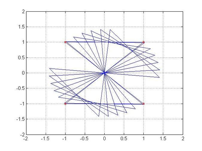
Example for Animation of a rotating shape
clc
clear
clf
point1=[ 1 1 ];
point2=[ -1 1 ];
point3=[ 1 -1 ];
point4=[ -1 -1 ];
plot(point1(1),point1(2),'*r')
hold on
plot(point2(1),point2(2),'*r')
hold on
plot(point3(1),point3(2),'*r')
hold on
plot(point4(1),point4(2),'*r')
axis([ -2 2 -2 2 ])
f=[ point2(1) point1(1)];
ff=[ point2(2) point1(2)];
f1=line(f,ff);
f=[ point2(1) point3(1)];
ff=[ point2(2) point3(2)];
f2=line(f,ff);
f=[ point3(1) point4(1)];
ff=[ point3(2) point4(2)];
f3=line(f,ff);
f=[ point4(1) point1(1)];
ff=[ point4(2) point1(2)];
f4=line(f,ff);
%hold on
grid on
for p=1:10:90;
theta=p*(pi/180);
R=[ cos(theta) -sin(theta); sin(theta) cos(theta)];
point11=point1*R;
point22=point2*R;
point33=point3*R;
point44=point4*R;
h=plot(point11(1),point11(2),'*r');
%hold on
h1=plot(point22(1),point22(2),'*r');
%hold on
h2=plot(point33(1),point33(2),'*r');
%hold on
h3=plot(point44(1),point44(2),'*r');
set(h,'EraseMode','xor')
set(h1,'EraseMode','xor')
set(h2,'EraseMode','xor')
set(h3,'EraseMode','xor')
set(h,'XData',point1(1),'YData',point1(2))
drawnow
set(h1,'XData',point2(1),'YData',point2(2))
drawnow
set(h2,'XData',point3(1),'YData',point3(2))
drawnow
set(h3,'XData',point4(1),'YData',point4(2))
drawnow
f=[ point22(1) point11(1)];
ff=[ point22(2) point11(2)];
f11=line(f,ff);
f=[ point22(1) point33(1)];
ff=[ point22(2) point33(2)];
f22=line(f,ff);
f=[ point33(1) point44(1)];
ff=[ point33(2) point44(2)];
f33=line(f,ff);
f=[ point44(1) point11(1)];
ff=[ point44(2) point11(2)];
f44=line(f,ff);
pause(1)
end
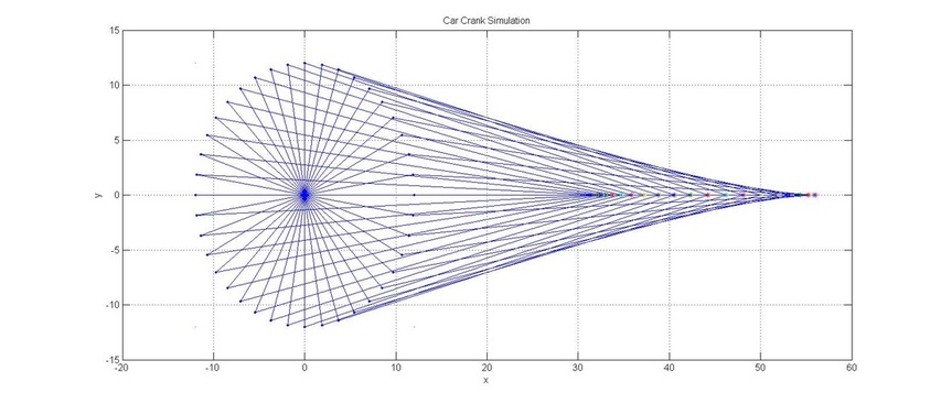
Example Modelling Reciprocating Engine
clc
clear
N=40;
R=12;
r=44;
%assigning a number to the output figure
figure(1)
% Generating the discrete angles and storing the angles in a matrix to
% retrive the data when ever needed
theta(1)=0;
for i=1:N;
theta(i+1)=theta(i)+9;
alpha(i)=(pi/180)*theta(i+1);
end
% Generating the two dimensional coordinates points, then storing
%the angles in a matrix to retrive the data when ever needed
for i=1:N;
x0(i)=R*cos(alpha(i));
y0(i)=R*sin(alpha(i));
end
%Allocating 4 points in the plotting domain to get the plot in a fixed
%domain , so that i wouldnt change while conducting the do loop.
plot(-12,12);
hold on
plot(-12,-12);
hold on
plot(60,12);
hold on
plot(12,-12);
grid on
title('Car Crank Simulation')
xlabel('x')
ylabel('y')
for i=1:N
plot(x0(i),y0(i),'.');
g=[ 0 x0(i)];
gg=[ 0 y0(i)];
%line linking between the center of coordinates and circual points
f=line(g,gg);
xx(i)=x0(i)+((r)^2-(y0(i)-0)^2)^0.5;
rr=[ x0(i) xx(i)];
rrr=[ y0(i) 0 ];
h=[ rr(2)-rr(1) rrr(2)-rrr(1) ];
%checking using the Phethagourus Therom that the length of the arm is
%constant
check(i)=norm(h);
%line linking between the circual points and piston
ff=line(rr,rrr);
plot(xx,0,'*')
hold on
%Assigning the pause command to an exponential function
tp(i)=exp(-0.001*i);
pause(tp(i))
end
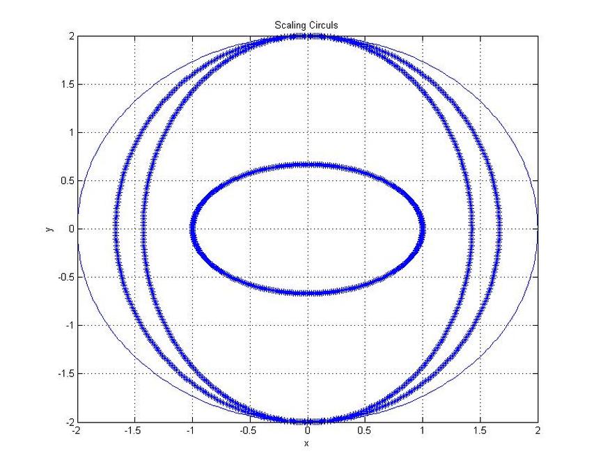
Example Scaling Shapes
clc
clear
r=2;
N=360;
theta(1)=0;
for i=1:N
theta(i+1)=theta(i)+1;
alpha(i)=(pi/180)*theta(i+1)
end
for i=1:N;
x(i)=r*cos(alpha(i));
y(i)=r*sin(alpha(i));
end
plot(x,y)
grid on
hold on
for i=1:N;
xx(i)=x(i)/1.2;
y(i)=r*sin(alpha(i));
end plot(xx,y,'*')
hold on
for i=1:N;
xx(i)=x(i)/1.4;
y(i)=r*sin(alpha(i));
end
plot(xx,y,'*')
hold on
for i=1:N;
xx(i)=x(i)/2;
yy(i)=y(i)/3;
end
plot(xx,yy,'*')
title('Scaling Circuls')
xlabel('x')
ylabel('y')
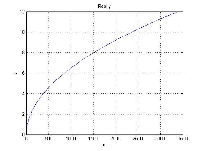
Grid Animation
clc clear M=30; N=40; L=12; x0=0; x1=x0+L; dx=L/M; xx=[ x0:dx:x1 ]; for j=1:N; for i=1:M; x(i,j)=xx(i); end end a(1)=0; for j=1:N; a(j+1)=a(j)+0.3; for i=1:M; x(i,j)=i*dx; y(i,j)=2*a(j)*(x(i,j))^2+2*x(i,j)-1; end end for j=1:N; plot(y(:,j),x(:,j)); grid on xlabel('x') ylabel('y') title('Really') MM(j) = getframe; end pause(3) figure(2) xlabel('x') ylabel('y') title('Really') frame_order = [1:N 2:1:N]; number_repeats = 1; movie(MM, [number_repeats frame_order]);
